
This post is part of my series on David Gauthier's Morals by Agreement
I am currently looking at Gauthier's proposed solution to the bargaining problem, something he calls minimax relative concession. The previous post outlined how to approach the bargaining problem and how to discover the MRC-solution. We can summarise it as follows:
- (1) Define the outcome space, i.e. all the feasible solutions to the bargaining game, and, if possible, draw it on an x-y axis.
- (2) Locate the initial bargaining position (IBP), i.e. the outcomes the parties could achieve without reaching agreement.
- (3) Locate the claim point, i.e. the point representing the maximum that each player can demand. This will usually be a point outside the outcome space, as players will initially demand more than can be distributed between them.
- (4) Let the players make concessions from this claim point and then compare the relative magnitude of those concessions.
- (5) The solution will be the point at which the maximum relative concession is as small as it is possible for it to be, hence the minimax relative concession.
In this post, we will look at two numerical examples of this solution-concept in action. These are discussed by Gauthier in Chapter 5.
1. Jane and Brian go to a Party
Jane has been invited to a party by Anne. She would really like to go but is worried that Brian might be there. She doesn't like him and would prefer not to go if he would be there. Brian has also been invited to the party, but he doesn't want to go unless Jane is going too.
Based on these preferences, we can draw-up the following payoff-table (or outcome matrix) for this game. The figures are interval measures of the utility each player derives from the four possible outcomes. They are measured by asking the players to consider lotteries over the different outcomes. For example, Jane's 2/3 payoff in the bottom left quadrant represents her indifference between that outcome and a lottery with a 2/3 chance of achieving her preferred outcome (top right) and a 1/3 chance of achieving her least favoured outcome (top left).

I won't get into it here, but it turns out that there is no pure strategy equilibrium in this game ("pure strategy" = definitely staying at home, or definitely going). There is, however, a mixed strategy equilibrium ("mixed strategy" = choosing the options with a certain probability).
Consider, if Jane chooses to go to the party with a probability of 1/4 (or 0.25) and to stay at home with a probability of 3/4 (or 0.75), then Bob's expected utilities from his possible choices will be:
- Stay at home: [(1/4 x 0) + (3/4 x 1/2)] = 3/8
- Go to the party: [(1/4 x 1) + (3/4 x 1/6)] = 3/8
Since the expected utilities from each option are the same, either response is utility maximising. A similar argument can be made for Jane's expected utilities if Brian chooses to stay at home with a probability of 1/2 and goes to the party with a probability of 1/2.
Consequently, the outcome resulting from the choice of these two mixed strategies is in equilibrium: each is a utility-maximising response to the other.
2. Jane and Bob Negotiate a Party-going Agreement
The analysis to this point has been straightforward game theory. Now we are going to look at the same outcome space through the lens of bargaining theory and try to locate the MRC solution.
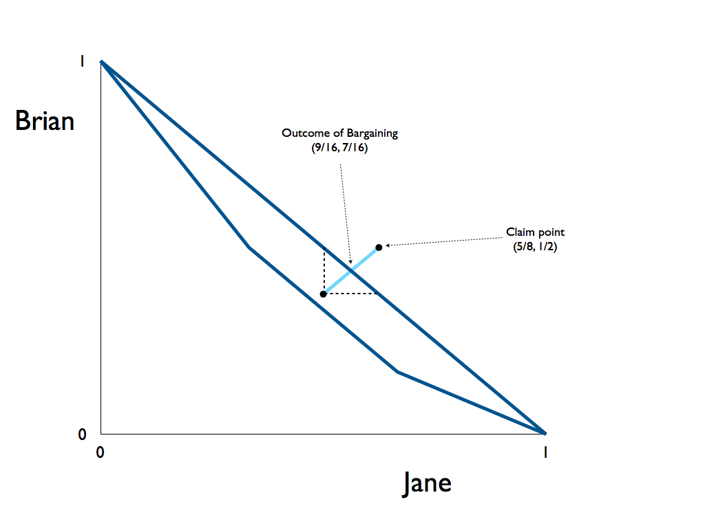
The first thing we need to is draw the outcome space and locate the initial bargaining position. In this case, the IBP will be the outcome that the parties could expect to obtain without an agreement. That will be the pair of outcomes associated with the mixed strategy equilibrium that has just been described, i.e. (1/2, 3/8).

Once we have drawn the outcome space and located the IBP, we can define the range of admissible outcomes that rational players would agree upon. These will occur on the optimal boundary (the line between (0, 1) and (1, 0)) between the points (1/2, 1/2) and (5/8, 3/8). Each party will initially try to claim as much as is possible. This means Brian will demand 1/2 and Jane will demand 5/8. This is illustrated below.
Obviously, the claim point is not an admissible outcome so the parties need to make some concessions. If we draw a straight line connecting the claim point to the IBP, then every point along that line will represent an equal relative concession from the players. This line intersects the optimal boundary at the point (9/16, 7/16). At this point, the relative concession for each player is 1/2 (I leave the math to the reader). This is the MRC-solution, because any outcome which gave more to Jane would force a greater relative concession from Brian and vice versa.
What does this solution mean in practice? Well, according to Gauthier, it means that Jane should be allowed to go to the party, and Brian should be allowed to play a mixed strategy with 7/16 probability of going to the party and 9/16 probability of staying at home.
3. Ernest and Adelaide Make a Deal
A second example works with monetary payoffs instead of utilities and allows us to explore the difference between relative concessions and absolute concessions.
Suppose that Ernest and Adelaide have the opportunity to co-operate in a mutually beneficial way, provided they can agree how to share their potential gains. Adelaide would receive a maximum net benefit of $500 from the joint venture, provided she receives all the gains after covering Ernest's costs. On the other hand, Ernest could only obtain a maximum net benefit of $50, provided he receives all the gains after covering Adelaide's costs. In this case we assume that neither can obtain anything without cooperation and so the IBP is (0, 0). We assume the possible outcomes lie along the curve in the following diagram.

Each party will initially claim as much as is possible for them to claim, i.e. the maximum net benefit. Obviously, this would not be desirable for the other party as they would then receive no gain from the joint enterprise. Concessions will have to be made by both sides.
Again, we follow the familiar method and draw a straight line connecting the claim point to the IBP. This line will intersect the optimal boundary of the outcome space at the point (353, 35). This amounts to an equal relative concession from each part of approximately 0.3. This is illustrated below.

Now the legitimate question arises: what about the absolute magnitudes of the gains and the concessions? Should they change how we think about the solution? After all, wouldn't Ernest be entitled to complain that he is not gaining anywhere near as much as Adelaide?
Here, we run into some interesting possibilities. Although Ernest could indeed make the complaint just outlined, Adelaide could also complain that, in the final agreement, Ernest is conceding far less than she is ($15 compared with $147). So, in some sense, the greater gain is offset by the greater loss.
Gauthier points out that this kind of absolute comparison is only possible in a few cases (where utilities map directly onto monetary outcomes). And in those cases, if we are tempted by some principle of equal gain, we should always bear in mind the principle of equal loss (as we just did). What makes MRC an acceptable solution to the bargaining problem is its ability to automatically balance relative loss and gain.
That's it for now. In the next post, we will try to relate the MRC-solution to the broader issues in moral and political philosophy that Gauthier is trying to address.
Your blog should come with a disclaimer. It is far too interesting and I have consequently lost several hours reading about things that are entirely irrelevant to the essay I am trying to write...
ReplyDeleteOn the other hand, your analysis of MRC is clear, concise and most importantly interesting so I am very grateful.
Well, thank you for the compliment. Hope you're focusing on that essay now...
ReplyDelete